exercise 11 :: Electronic structure of graphene and its Wannierization

The exercise demonstrates calculation of electronic band structure of graphene and maximally localized Wannier functions (MLWF) using wannier90 package.

TASK 01

Consider graphene with nearest neighbor carbon atom distance of 1.42 Angstrom and sheet separation of 12 Angstrom in order to model a single sheet. The input for scf calculations could look like:

 &control
	title = 'graphene, c=12 AA vacuum' ,
	calculation = 'scf' ,
	restart_mode = 'from_scratch' ,
	outdir = './tmp/' ,
	pseudo_dir = './' ,
	prefix = 'graphene' ,
	verbosity = 'high' ,
	/
&system
	ibrav = 4,
	celldm(1) = 4.647806, celldm(3) = 4.87901473571,
	occupations = 'smearing', smearing = 'm-v', degauss = 0.0001,
	nat = 2,
	ntyp = 1,
	ecutwfc = 40, ecutrho = 160 ,
	nbnd = 16,
	/
&electrons
	conv_thr = 1.0d-8,
	/
ATOMIC_SPECIES
   C   12.01078  C.pbe-mt_fhi.UPF
ATOMIC_POSITIONS crystal
	C      0.333333333    0.666666667    0.000000000
	C      0.666666667    0.333333333    0.000000000
K_POINTS automatic
	12 12 1   0 0 0

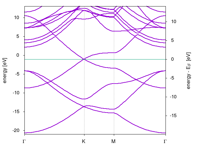
Perform scf calculations to obtain ground state electronic density and then perform bands calculations along high symmetry lines connecting K-$\Gamma$-M-K points in first Brillouin zone. For coordinates of the high symmetry points see this website. The resulting band structure is show in the following figure.

TASK 02

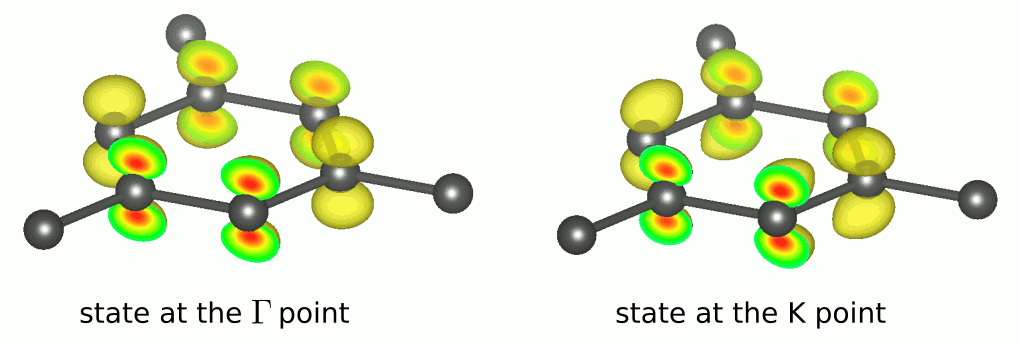
Investigate electronic states forming the occupied band that crosses at the K point in the so called Dirac point. For this purpose calculate electronic density in real space for the state at the $\Gamma$ point for energy of about -7.5 eV below the Fermi energy, and for the K point state at the Fermi energy. For this purpose perform nscf calculations for the $\Gamma$ and K points only specifying:

K_POINTS crystal 
  2
0.00000000   0.00000000   0.0   1 
0.33333333   0.33333333   0.0   1

The output file should contain the following information

	k = 0.0000 0.0000 0.0000 (  1833 PWs)   bands (ev):

-20.6556  -8.7365  -4.1598  -4.1598   2.1188   3.2694   4.0444   7.2084
 7.2614   7.2614   8.4672  10.4427  11.4584  13.4540  15.2730  21.4718

occupation numbers
 1.0000   1.0000   1.0000   1.0000   0.0000   0.0000   0.0000   0.0000
 0.0000   0.0000   0.0000   0.0000   0.0000   0.0000   0.0000   0.0000

	k = 0.3333 0.5774 0.0000 (  1779 PWs)   bands (ev):
-13.6864 -13.6864 -11.6861  -1.0728  -1.0728   9.5744  11.8605  11.8605
12.4498  14.0514  14.0514  14.1746  14.1746  14.5703  15.2441  15.7374

occupation numbers
 1.0000   1.0000   1.0000   0.5000   0.5000   0.0000   0.0000   0.0000
 0.0000   0.0000   0.0000   0.0000   0.0000   0.0000   0.0000   0.0000

 the Fermi energy is    -1.0726 ev

Where you can see that we are interested for the second state at the $\Gamma$ point fourth state at the K point. Now we are about to perform the electronic density plot in real space using pp.x program. The input for the electronic density of the state at $\Gamma$ at energy about -7.5 eV could look like:

 &inputpp
    prefix  = 'graphene'
    outdir='./tmp/',
    filplot = 'tmp.G2',
    plot_num = 7,
    spin_component = 0,
    kpoint(1) = 1,
    kband(1) = 2,
    kband(2) = 2,
 /
 &plot
   nfile=1
   filepp(1)='tmp.G2', weight(1)=1.0
   iflag=3
   output_format=3
   e1(1)=1.0, e1(2)=0.0,     e1(3)=0.0
   e2(1)=0.0, e2(2)=1.73205, e2(3)=0.0
   e3(1)=0.0, e3(2)=0.0,     e3(3)=1.0
   x0(1)=0.0, x0(2)=0.0,     x0(3)=-0.5
   nx=60, ny=110, nz=60
   fileout='edp_G-point_E-7.5eV.xsf'
 /

For further input description see the link. Similarly you can calculate electronic density in real space for the state at the fourth band at the K point. Obtained xsf files can be visualized, e.g., with VESTA providing the following plots. One can see that both the states are similar to atomic $p_z$ orbital suggesting that the band is formed by the conjugate $\pi$-electrons of carbon.

TASK 03

Wannierize the $\pi$-bands of graphene using Wannier90 package.

1. perform nscf calculation with setting the following flag: wf_collect = .true.; nosym = .true. in the input file for k-points generated on grid using kmesh utility:
   $PATH_TO_WANNIER90_CODE/utility/kmesh.pl 12 12 1 and use the k-point list placing it to the K_POINTS block of your nscf input file.

2. pre-process for Wannierization. Use provided example input file for wannier90. For further details of the input flags refer to user guide.

      !---------------------------GENERAL
      num_bands        =  16
      num_wann         =  2
      !------------------------------CONV
      iprint = 3
      num_iter         = 500
      num_print_cycles = 50
      !!! -- Disentanglement parameters -- !!!
      dis_froz_min     = -3.0
      dis_froz_max     = 2.0
      dis_win_min      = -10.0
      dis_win_max      = 11.0
      !-----------------------------bands
      !restart = plot
      bands_plot = .true.
      !wannier_plot = .false.
      write_hr = .true.
   
      begin kpoint_path
        G  0.0       0.0       0.0     K  0.333333  0.333333  0.0
        K  0.333333  0.333333  0.0     M  0.5       0.0       0.0
        M  0.5       0.0       0.0     G  0.0       0.0       0.0
      end kpoint_path
      !----------------------------SYSTEM
      begin unit_cell_cart
      bohr
         4.647806   0.000000   0.000000  
        -2.323903   4.025118   0.000000
         0.000000   0.000000  22.676715
      end unit_cell_cart
   
      begin atoms_frac
          C      0.333333333    0.666666666    0.000000000    
          C      0.666666666    0.333333333    0.000000000    
      end atoms_frac
   
      begin projections
      	C:pz
      end projections
   
      spinors = false
   
      !----------------------------KPOINTS
      mp_grid : 12 12 1
   
      begin kpoints
        0.00000000  0.00000000  0.00000000 
        0.00000000  0.08333333  0.00000000 
        0.00000000  0.16666667  0.00000000 
        . . .  {k point coordinates are those generated by the kmesh.pl}
      end kpoints
   

   The num_bands, num_wann, unit_cell_cart and atoms_frac can be taken from the scf or nscf output files. For projections we consider the $p_z$ orbitals and mp_grid should be the same list as used for nscf calculations generated by the kmesh.pl 12 12 1 wan script. Save the above input as case.win.
   Run the pre-processing: wannier90.x -pp case to generate case.nnkp file needed for further step.

3. Run pw2wannier.x < pw2wann.in > out.pw2wan to compute overlaps between the Bloch states and the projections of the starting guess (written in the case.mmn and case.amn files). The input file pw2wann.in should look like:

   &inputpp 
      outdir = './tmp'
      prefix = 'graphene'
      seedname = 'case'
      write_mmn = .true.
      write_amn = .true.
      write_spn = .true.
      write_unk = .false.
   /
   

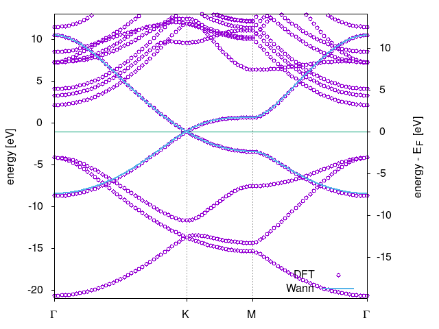
4. Perform Wannierization by computing the MLWFs: wannier90.x case. Check your Wannierization by plotting the case_band.dat over the DFT band structure. In the figure below the Wannierized energy dispersions of the $\pi$-bands are shown with (blue) lines over the DFT data (open circles).
   

---

Martin Gmitra :: martin.gmitra@upjs.sk
This work is licensed under a Creative Commons Attribution 4.0 International License.